Double Declining Balance Depreciation: Formula, Example and Excel DDB
Master double declining balance depreciation: DDB formula, full worked example with the SLN switch rule, Excel =DDB() function, and when to use accelerated depreciation.

ACA | FMVA® | 19 Years in Finance
A technology company books a USD 20,000 server. Straight-line over 5 years: USD 4,000 per year. By Year 2, the book value is USD 16,000. The market value of that server is USD 9,000. The book value overstates economic reality by 78%.
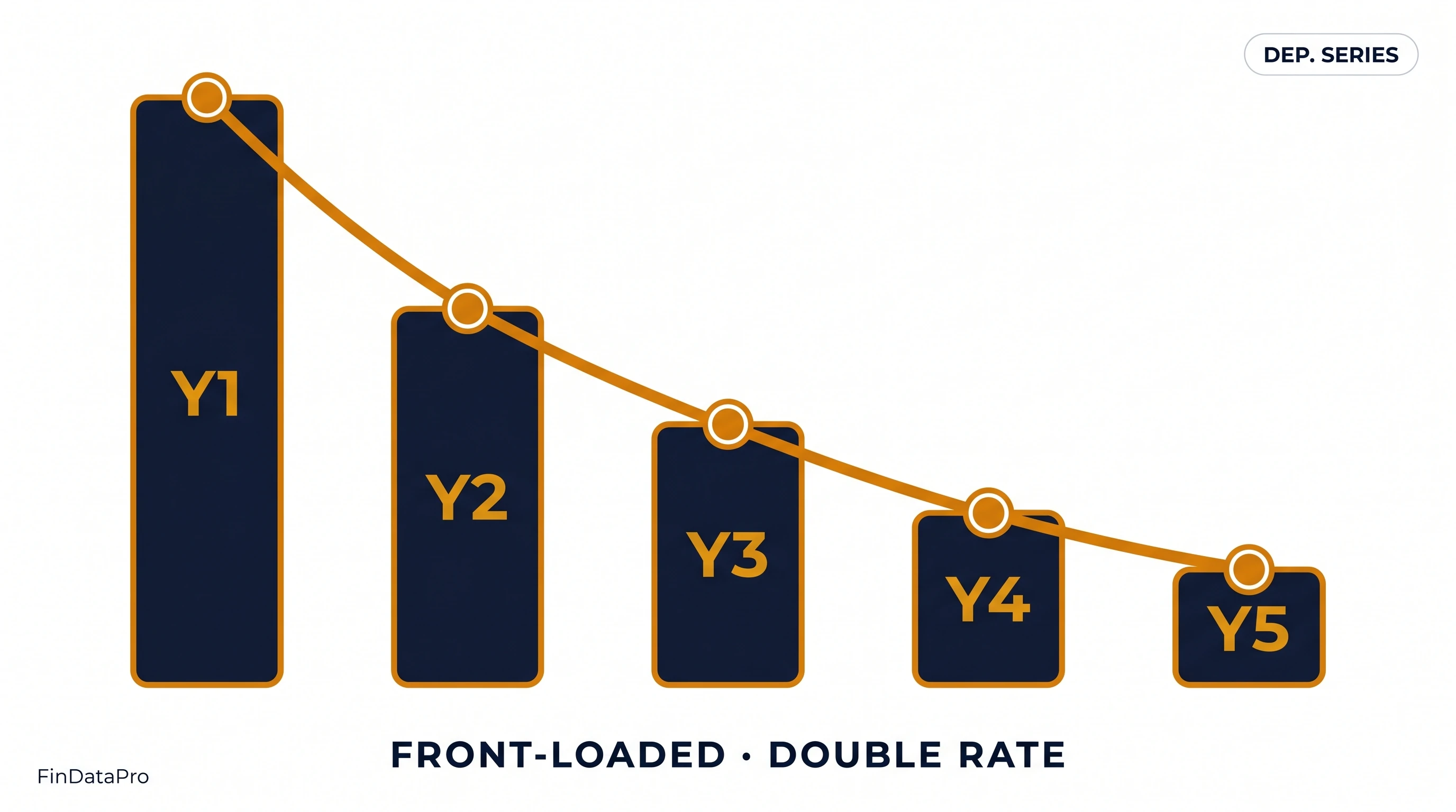
This is the problem that double declining balance depreciation is designed to address. The method front-loads the depreciation charge into the years when the asset is delivering its highest economic value and losing its market value most rapidly. The P&L charge tracks the economic consumption of the asset rather than the calendar.
DDB is not universally appropriate. For assets that wear out evenly, straight-line is more accurate. For assets that degrade sharply in early years: technology, certain vehicles, production machinery with high initial output: DDB produces a depreciation schedule that better matches what is actually happening to the asset's value.
Table of Contents {#toc}
- What Is Double Declining Balance Depreciation
- The DDB Formula
- The Switch-to-Straight-Line Rule
- Step-by-Step Worked Example
- Full DDB Schedule with Switch Point
- Excel Implementation: The =DDB() Function
- IAS 16 Compliance for DDB
- When DDB Is the Right Choice (and When It Is Not)
- DDB and Deferred Tax
- Frequently Asked Questions
- Conclusion
What Is Double Declining Balance Depreciation {#what-is-ddb}
Double declining balance is an accelerated depreciation method. It applies a rate equal to twice the straight-line rate to the declining book value of the asset each period. The charge is highest in the first period and declines progressively in subsequent periods because the rate is fixed but the book value it applies to shrinks each year.
The "double" in double declining balance refers to the factor: 2 times the straight-line rate. The straight-line rate for a 5-year asset is 20% (1/5). Double declining balance applies 40% (2 × 20%).
Two features distinguish DDB from straight-line:
- The rate applies to the book value (not the original cost)
- Salvage value is not subtracted before applying the rate: it only acts as a floor (the book value cannot fall below the salvage)
Both distinctions matter mechanically. The first means the base shrinks each year. The second means Year 1 depreciation is 40% of the full cost: not 40% of (cost minus salvage). This front-loading effect is more pronounced than in WDV methods where the residual value does affect the rate derivation.
The DDB Formula {#formula}
DDB Rate = 2 / Useful Life
Period Depreciation = Opening Book Value × DDB Rate
The rate is fixed for the entire useful life. The charge declines each year because the opening book value shrinks.
Floor rule: In any period, the depreciation charge is capped so the closing book value does not fall below the salvage value.
The Switch-to-Straight-Line Rule {#switch-rule}
This is the rule that most DDB explanations either skip or explain inadequately. Without the switch, DDB does not bring the book value down to the salvage value by the end of the asset's useful life.
The mechanism:
In the later periods of an asset's life, the DDB charge (40% of a small book value) becomes smaller than the straight-line charge needed to bring the book value to the salvage value by the final year. At the crossover point, the method switches to straight-line.
How to identify the switch point:
At the end of each period, compare:
- DDB charge for the next period: opening book value × DDB rate
- SLN charge for remaining periods: (opening book value - salvage) / remaining years
When SLN charge exceeds DDB charge: switch to SLN from that period forward.
Excel's =DDB() function handles this switch automatically. Manual schedules must include the comparison logic in each row. Omitting it produces a book value above the salvage at the end of Year N: an error.
Step-by-Step Worked Example {#worked-example}
Asset: IT equipment
| Input | Value |
|---|---|
| Cost | USD 20,000 |
| Salvage value | USD 2,000 |
| Useful life | 5 years |
| DDB Rate | 2 / 5 = 40% |
Year 1:
- Opening book value: USD 20,000 (full cost)
- DDB charge: 20,000 × 40% = USD 8,000
- Closing book value: USD 12,000
Year 2:
- Opening book value: USD 12,000
- DDB charge: 12,000 × 40% = USD 4,800
- SLN check: (12,000 - 2,000) / 4 = USD 2,500. DDB (4,800) > SLN (2,500): stay DDB
- Closing book value: USD 7,200
Year 3:
- Opening book value: USD 7,200
- DDB charge: 7,200 × 40% = USD 2,880
- SLN check: (7,200 - 2,000) / 3 = USD 1,733. DDB (2,880) > SLN (1,733): stay DDB
- Closing book value: USD 4,320
Year 4:
- Opening book value: USD 4,320
- DDB charge: 4,320 × 40% = USD 1,728
- SLN check: (4,320 - 2,000) / 2 = USD 1,160. DDB (1,728) > SLN (1,160): stay DDB
- Closing book value: USD 2,592
Year 5:
- Opening book value: USD 2,592
- DDB charge: 2,592 × 40% = USD 1,037
- SLN check: (2,592 - 2,000) / 1 = USD 592. DDB (1,037) > SLN (592): switch to SLN
- Charge applied: USD 592
- Closing book value: USD 2,000 (= salvage value)
The switch happens in Year 5. The DDB charge of USD 1,037 would overshoot the salvage value. The correct charge is USD 592.
Full DDB Schedule with Switch Point {#full-schedule}
| Year | Opening BV (USD) | DDB Charge (USD) | SLN Check (USD) | Method Applied | Closing BV (USD) |
|---|---|---|---|---|---|
| 1 | 20,000 | 8,000 | : | DDB | 12,000 |
| 2 | 12,000 | 4,800 | 2,500 | DDB | 7,200 |
| 3 | 7,200 | 2,880 | 1,733 | DDB | 4,320 |
| 4 | 4,320 | 1,728 | 1,160 | DDB | 2,592 |
| 5 | 2,592 | 1,037 | 592 | SLN | 2,000 |
| Total | 18,000 |
Total depreciation: USD 18,000 = Cost (20,000) - Salvage (2,000). The depreciable amount is fully allocated by the end of Year 5.
Compare to straight-line: USD 3,600 per year for 5 years = USD 18,000. Same total. Completely different timing.
Excel Implementation: The =DDB() Function {#excel}
Excel's =DDB() function handles double declining balance depreciation, including the switch to straight-line at the crossover point.
Syntax:
=DDB(cost, salvage, life, period, [factor])
| Argument | Description |
|---|---|
| cost | Asset acquisition cost |
| salvage | Residual / salvage value |
| life | Useful life in periods |
| period | The period to calculate (1, 2, 3...) |
| [factor] | Declining balance factor: default is 2 (double declining). Use 1.5 for 150% declining balance. |
Applied to the worked example:
| Formula | Output (USD) |
|---|---|
=DDB(20000, 2000, 5, 1) | 8,000 |
=DDB(20000, 2000, 5, 2) | 4,800 |
=DDB(20000, 2000, 5, 3) | 2,880 |
=DDB(20000, 2000, 5, 4) | 1,728 |
=DDB(20000, 2000, 5, 5) | 592 |
The function automatically applies the switch in Year 5: returning 592 rather than the DDB charge of 1,037 that would overshoot the salvage. You do not need to code the switch logic manually when using =DDB().
Building a full schedule in Excel:
Set up a table with period numbers in Column A. In the depreciation column, reference: =DDB($B$2,$B$3,$B$4,A[row]) with absolute references for cost, salvage, and life. The function handles the switch automatically.
The =VDB() alternative:
For schedules that require a switch to straight-line without Excel's built-in DDB logic, or for non-standard periods, use =VDB(cost, salvage, life, start_period, end_period, [factor], [no_switch]). Setting [no_switch] to FALSE allows the switch; TRUE forces DDB throughout. VDB is more flexible but requires start/end period inputs rather than a single period number.
Building depreciation schedules manually for multiple assets with DDB, tracking the switch point in each asset's schedule, and reconciling against the tax position: this is where Excel-based approaches accumulate the most version and formula drift. DepreciationLab automates DDB schedules with the switch-to-SLN logic built in for every asset, eliminating the need to maintain switch-point logic per asset. Try DepreciationLab at depreciationlab.org.
IAS 16 Compliance for DDB {#ias16}
IAS 16 permits double declining balance. The standard requires the depreciation method to reflect the pattern of economic benefit consumption from the asset. DDB satisfies this requirement when the asset genuinely delivers more benefit in early years.
The consistency requirement:
Once selected, the method must be applied consistently to all assets of the same class. You cannot apply DDB to some computers and straight-line to others. Within an asset class, the method is uniform.
The annual review obligation:
IAS 16.61 requires the depreciation method to be reviewed at each financial year-end. If the consumption pattern has changed: for example, if technology assets are being retained and upgraded rather than replaced every 3 years: the method should be reviewed and changed if necessary. A change in method is a change in accounting estimate under IAS 8, applied prospectively.
What the review documentation must show:
Evidence that the current method continues to reflect the pattern of benefit consumption. For DDB, this typically means evidence that the asset class loses significant value in early years and that economic utility declines at a faster-than-linear rate. For technology assets in the GCC, where replacement cycles have been extending due to capital constraints in recent years, this is a review worth conducting properly.
The full IAS 16 standard is at ifrs.org.
When DDB Is the Right Choice (and When It Is Not) {#when-to-use}
Use DDB when:
The asset is a technology asset with rapid obsolescence: servers, workstations, point-of-sale systems, specialised software implementations. The asset is a vehicle type where market value declines sharply in the first two years. The asset is production machinery where maximum capacity and efficiency are delivered early and decline with wear. The entity is seeking to front-load depreciation expense for legitimate economic reasons: not tax positioning (which is a separate calculation).
Do not use DDB when:
The asset has a stable, uniform consumption pattern: long-life buildings, office furniture, leasehold improvements. The asset's useful life is driven by time-based factors rather than wear or obsolescence. The entity cannot demonstrate that the DDB rate matches the actual rate of economic benefit decline: in which case a WDV method with a lower rate may be more appropriate than double declining.
DDB vs WDV (Companies Act):
DDB uses a rate of 2/life, applied to the full book value without a residual value floor in the rate formula. WDV under the Companies Act derives its rate from the useful life AND the 5% residual value, producing a lower rate for the same life. For a 5-year asset: DDB rate = 40%; WDV rate (at 5% residual) = 45.07%. WDV actually produces higher Year 1 depreciation for short-life assets. The key structural difference is the floor treatment and the rate derivation.
DDB and Deferred Tax {#deferred-tax}
In most jurisdictions, tax depreciation uses a different method or rate from the accounting DDB charge. The difference creates a deferred tax position under IAS 12.
For IFRS reporting entities in the GCC:
If the accounting method is DDB and the jurisdiction uses a straight-line or prescribed rate for tax purposes, the timing difference reverses over the asset's life. In early years, DDB book depreciation exceeds tax depreciation: a deferred tax liability arises. In later years, when the DDB charge has dropped below the SLN equivalent and the SLN switch has occurred, book depreciation may fall below tax depreciation, and the deferred tax liability reverses.
For Indian entities using DDB:
The comparison is more complex: book depreciation under DDB vs the Income Tax Act block-of-assets WDV rate. The direction of the timing difference depends on whether the applicable Income Tax rate (e.g., 15% for plant and machinery) is higher or lower than the effective DDB rate for the asset class.
In all cases, the deferred tax arising from depreciation timing differences is a balance sheet item under IAS 12: not a footnote disclosure. It requires a separate tracking schedule that mirrors the depreciation schedule but applies the IAS 12 methodology.
Frequently Asked Questions {#faq}
What is double declining balance depreciation?
DDB is an accelerated method that applies twice the straight-line rate to the declining book value each period. For a 5-year asset, the rate is 40% (2/5). The charge is highest in Year 1 and declines each year. Total depreciation equals the depreciable amount: only the timing differs from straight-line.
When should I use double declining balance instead of straight-line?
When the asset delivers most of its economic value in early years: technology, vehicles with rapid early depreciation, production machinery. DDB matches the depreciation charge to the period of highest economic benefit. It is not appropriate for assets with stable, even consumption across their useful life.
What is the Excel formula for double declining balance?
=DDB(cost, salvage, life, period, [factor]). Factor defaults to 2. Example: =DDB(20000, 2000, 5, 1) returns 8,000. The function applies the switch-to-SLN rule automatically when the SLN charge exceeds the DDB charge.
What is the DDB switch-to-straight-line rule?
In any period where the remaining SLN charge (book value minus salvage, divided by remaining years) exceeds the DDB charge, the method switches to SLN. This prevents the book value from remaining above the salvage value at the end of the asset's life. Excel's =DDB() handles this automatically. Manual schedules need the comparison logic in each row.
Is double declining balance permitted under IFRS?
Yes. IAS 16 permits DDB when it reflects the pattern of economic benefit consumption from the asset. It must be applied consistently within an asset class and reviewed annually.
Does double declining balance always give the lowest book value?
In the early years, yes. By the end of the useful life, all methods converge to the same salvage value. DDB produces higher cumulative depreciation in the first half of an asset's life and lower in the second half. The total is the same as straight-line.
What is the difference between DDB and 150% declining balance?
DDB uses a factor of 2 (200% of straight-line). 150% declining balance uses a factor of 1.5. In Excel: =DDB(cost, salvage, life, period, 1.5) produces 150% declining balance. The 150% method was used in some US tax contexts under the pre-MACRS regime.
Conclusion {#conclusion}
Double declining balance is the most aggressive standard accounting depreciation method available. For assets that lose value rapidly in the first few years: technology, vehicles, high-output machinery: it produces a depreciation schedule that reflects the economic reality of the asset far better than straight-line.
The switch-to-straight-line rule is not optional. Miss it and the book value at the end of Year 5 is above the salvage value: an error in every year's closing balance from the switch point onwards.
Building and maintaining DDB schedules with the switch logic for every affected asset in a register, and keeping the deferred tax calculation in parallel, is where annual depreciation workings most frequently break down in mid-size finance teams.
DepreciationLab handles DDB schedules with the switch rule applied automatically for every asset, alongside the deferred tax position tracking. No formula drift. No missed switch points.
Part of the FinDataPro Depreciation Methods Series. Related posts:
- The Complete Guide to All 7 Depreciation Methods (Pillar)
- Straight-Line Depreciation: Formula, Example and Excel
- WDV Depreciation: Companies Act 2013: Schedule II and Rate Derivation
- Free Fixed Asset Depreciation Calculator (Excel)
⚡Try It Yourself
Calculate double declining balance depreciation and see the switch point automatically. Calculate now at Depreciation Lab →
Prashant Panchal is a Chartered Accountant (ACA) and Financial Modelling & Valuation Analyst (FMVA®) with 19 years of experience in finance, FP&A, and financial modelling across the GCC region. He is the founder of FinDataPro.
Discussion
Leave a Comment
Comments are moderated and appear once approved.